From ISLR
At a recent data science meetup in Houston, I spoke to one of the panel speakers who was a data scientist for an oil and gas consulting company. They mostly used tree based methods like random forest, bagging and boosting and one of the challenges he said they frequently encountered while presenting their results, were putting confidence intervals on the variable importance measures.
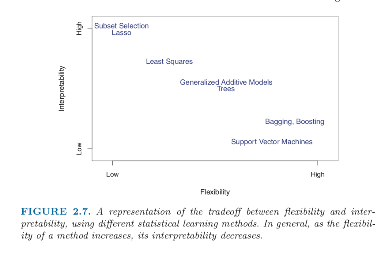
Often times, industry experts would not only like good predictive models but at the same time, models that are somewhat interpretable. It reminds me of a very useful graphic from the ISLR book (An excellent book by the way for anyone who hasn’t yet read it)
From ISLR
As you can see, tree based methods are highly flexible (and thus, potential to have better predictions) but low on the interpretability scale.
I sought out to look for recent papers and techniques to try to interpret random forest algorithms. A recent publication by Dr. Hemant Ishwaran sought out to do just this https://onlinelibrary.wiley.com/doi/abs/10.1002/sim.7803
Below I’ll be implementing the techniques in this paper using the randomForestSRC package on the ever famous Ames housing dataset!
Import the required libraries
library(tidyverse)
library(naniar)
library(caret)
library(e1071)
library(ranger)
library(corrplot)
Import the training data (downloaded from [kaggle] https://www.kaggle.com/datasets)
train <- read_csv("/Users/dilsherdhillon/Documents/Website/DilsherDhillon/static/files/train.csv")The package naniar provides a nice feature which can be utilized to visualize completeness of data in one simple line of code
gg_miss_var(train,show_pct = TRUE)
## Other functions that maybe useful for your specific problem
#vis_miss(train,show_perc_col = TRUE,warn_large_data = TRUE)
#vis_miss(train,show_perc_col = TRUE,warn_large_data = TRUE)
#miss_case_table(train)
The plot shows ~17% data missing for ‘Lot Frontage’, and ‘Alley’,‘PoolQC’,‘Fence’ and ‘MiscFeatures’ are missing >70% of their data. About ~48% of the ‘FireplaceQU’ variable is missing.
At this point it would suffice to say we should remove all these variables except lot frontage. Since this tutorial is more focused towards showcasing how to put confidence intervals on variable importance for RandomForest models, we’ll work with data that is complete and not worry too much about data imputation etc.
For imputation of missing data, the MICE package in R and the corresponding text serves as a excellent resource for the interested reader
Remove variables with high % of missing data
dta<-train%>%
select(-c(Alley,FireplaceQu,PoolQC,Fence,MiscFeature,Id,LotFrontage))Before we start implementing the random forest model, it’s a good idea to run some quality checks on the variables. We know how the saying goes, garbage in, garbage out. One of these is checking for variables that have near zero variance - they are essentially the same for all samples and would simply add unwanted noise to our model.
The caret package has a nice function that lets us check for variables that may have zero or near zero variance
nzv<-nearZeroVar(dta,saveMetrics = TRUE)
nzv
## freqRatio percentUnique zeroVar nzv
## MSSubClass 1.792642 1.0273973 FALSE FALSE
## MSZoning 5.279817 0.3424658 FALSE FALSE
## LotArea 1.041667 73.4931507 FALSE FALSE
## Street 242.333333 0.1369863 FALSE TRUE
## LotShape 1.911157 0.2739726 FALSE FALSE
## LandContour 20.809524 0.2739726 FALSE TRUE
## Utilities 1459.000000 0.1369863 FALSE TRUE
## LotConfig 4.000000 0.3424658 FALSE FALSE
## LandSlope 21.261538 0.2054795 FALSE TRUE
## Neighborhood 1.500000 1.7123288 FALSE FALSE
## Condition1 15.555556 0.6164384 FALSE FALSE
## Condition2 240.833333 0.5479452 FALSE TRUE
## BldgType 10.701754 0.3424658 FALSE FALSE
## HouseStyle 1.631461 0.5479452 FALSE FALSE
## OverallQual 1.061497 0.6849315 FALSE FALSE
## OverallCond 3.257937 0.6164384 FALSE FALSE
## YearBuilt 1.046875 7.6712329 FALSE FALSE
## YearRemodAdd 1.835052 4.1780822 FALSE FALSE
## RoofStyle 3.989510 0.4109589 FALSE FALSE
## RoofMatl 130.363636 0.5479452 FALSE TRUE
## Exterior1st 2.319820 1.0273973 FALSE FALSE
## Exterior2nd 2.355140 1.0958904 FALSE FALSE
## MasVnrType 1.941573 0.2739726 FALSE FALSE
## MasVnrArea 107.625000 22.3972603 FALSE FALSE
## ExterQual 1.856557 0.2739726 FALSE FALSE
## ExterCond 8.780822 0.3424658 FALSE FALSE
## Foundation 1.020505 0.4109589 FALSE FALSE
## BsmtQual 1.050162 0.2739726 FALSE FALSE
## BsmtCond 20.169231 0.2739726 FALSE TRUE
## BsmtExposure 4.312217 0.2739726 FALSE FALSE
## BsmtFinType1 1.028708 0.4109589 FALSE FALSE
## BsmtFinSF1 38.916667 43.6301370 FALSE FALSE
## BsmtFinType2 23.259259 0.4109589 FALSE TRUE
## BsmtFinSF2 258.600000 9.8630137 FALSE TRUE
## BsmtUnfSF 13.111111 53.4246575 FALSE FALSE
## TotalBsmtSF 1.057143 49.3835616 FALSE FALSE
## Heating 79.333333 0.4109589 FALSE TRUE
## HeatingQC 1.731308 0.3424658 FALSE FALSE
## CentralAir 14.368421 0.1369863 FALSE FALSE
## Electrical 14.191489 0.3424658 FALSE FALSE
## 1stFlrSF 1.562500 51.5753425 FALSE FALSE
## 2ndFlrSF 82.900000 28.5616438 FALSE FALSE
## LowQualFinSF 478.000000 1.6438356 FALSE TRUE
## GrLivArea 1.571429 58.9726027 FALSE FALSE
## BsmtFullBath 1.455782 0.2739726 FALSE FALSE
## BsmtHalfBath 17.225000 0.2054795 FALSE FALSE
## FullBath 1.181538 0.2739726 FALSE FALSE
## HalfBath 1.706542 0.2054795 FALSE FALSE
## BedroomAbvGr 2.245810 0.5479452 FALSE FALSE
## KitchenAbvGr 21.415385 0.2739726 FALSE TRUE
## KitchenQual 1.254266 0.2739726 FALSE FALSE
## TotRmsAbvGrd 1.221884 0.8219178 FALSE FALSE
## Functional 40.000000 0.4794521 FALSE TRUE
## Fireplaces 1.061538 0.2739726 FALSE FALSE
## GarageType 2.248062 0.4109589 FALSE FALSE
## GarageYrBlt 1.101695 6.6438356 FALSE FALSE
## GarageFinish 1.433649 0.2054795 FALSE FALSE
## GarageCars 2.233062 0.3424658 FALSE FALSE
## GarageArea 1.653061 30.2054795 FALSE FALSE
## GarageQual 27.312500 0.3424658 FALSE TRUE
## GarageCond 37.885714 0.3424658 FALSE TRUE
## PavedDrive 14.888889 0.2054795 FALSE FALSE
## WoodDeckSF 20.026316 18.7671233 FALSE FALSE
## OpenPorchSF 22.620690 13.8356164 FALSE FALSE
## EnclosedPorch 83.466667 8.2191781 FALSE TRUE
## 3SsnPorch 478.666667 1.3698630 FALSE TRUE
## ScreenPorch 224.000000 5.2054795 FALSE TRUE
## PoolArea 1453.000000 0.5479452 FALSE TRUE
## MiscVal 128.000000 1.4383562 FALSE TRUE
## MoSold 1.081197 0.8219178 FALSE FALSE
## YrSold 1.027356 0.3424658 FALSE FALSE
## SaleType 10.385246 0.6164384 FALSE FALSE
## SaleCondition 9.584000 0.4109589 FALSE FALSE
## SalePrice 1.176471 45.4109589 FALSE FALSEdim(nzv)## [1] 74 4There seem to be predictors with very low variance - we use the default metrics here to assesss whether we classify a predictor as near zero-variance or not
nzv<-nearZeroVar(dta) ## don't save metrics here since we need the index of the near zero variance variables
dta_v2<-dta[,-nzv]
dim(dta_v2)
## [1] 1460 5420 variables with near zero variance were removed
Another quick measure we should look at is multi-collinearity.
Check for correlations between the numeric variables to avoid multi-collinearity issues
dta_v2%>%
  select_if(.,is.integer)%>%
  cor(.,use="pairwise.complete.obs",method="spearman")%>%
    corrplot(., type = "upper",method="circle",title="Spearman  Correlation",mar=c(0,0,1,0),number.cex = .2)
Some very interesting things come out from the plot above. We see that the variable ‘YearBuilt’ is very highly correlated with ‘GarageYrBuilt’ - which makes sense. It’s likely that the garage for the house was built as the same time as the house was built. Similarly, GarageCars is highly correlated with GarageArea which again makes sense - more the area, more cars can be parked in the garage.
An encouraging thing that does come out is several of the variables are somewhat moderate to high correlated with the sale price.
We see that there are some variables that are actually categorical in nature, but are treated as integers/numbers - they should really be converted to categorical variables. For example, MoSold is the month of the year in which the house was sold from 1… through 12. In addition, the character vectors need to be converted to factors as well to be used in the random forest model.
dta_v2<-dta_v2%>%
  mutate_at(.,vars(MSSubClass,MoSold,BsmtFullBath,BsmtHalfBath,FullBath,HalfBath,YrSold),as.factor)%>%
  map_if(is.character,as.factor)%>%
  as.tibble()
## Warning: `as.tibble()` is deprecated, use `as_tibble()` (but mind the new semantics).
## This warning is displayed once per session.How many predictors have correlation >0.80?
dta_v2%>%
  select_if(.,is.integer)%>%
  cor(.,method="spearman",use="pairwise.complete.obs")%>%
  findCorrelation(.,cutoff = 0.80)
## [1] 21 12 17 4 9How many have >0.90
dta_v2%>%
  select_if(.,is.integer)%>%
  cor(.,method="spearman",use="pairwise.complete.obs")%>%
  findCorrelation(.,cutoff = 0.90)
## integer(0)No predictors have correlation >0.90
A random forest model for training in caret needs complete data - in cases where the specified method can handle missing data, using the argument ‘na.action=na.pass’ in the train function (look up documentation in caret to which models can work with missing date)
But for our purposes, we drop all cases with any missing values
dta_rf<-dta_v2%>%
  drop_na()
dim(dta_rf)
## [1] 1339 54We’re down to 1339 samples from 1460 originally
Let’s fit a vanilla random forest model. The default option in caret runs the specified model over 25 bootstrap samples across 3 options of the mtry tuning parameter.
rf_vanilla<-train(log(SalePrice)~.,method="ranger",data=dta_rf)
rf_vanilla
## Random Forest
##
## 1339 samples
## 53 predictor
##
## No pre-processing
## Resampling: Bootstrapped (25 reps)
## Summary of sample sizes: 1339, 1339, 1339, 1339, 1339, 1339, ...
## Resampling results across tuning parameters:
##
## mtry splitrule RMSE Rsquared MAE
## 2 variance 0.2107885 0.7992672 0.14917042
## 2 extratrees 0.2282024 0.7586043 0.16510928
## 104 variance 0.1366434 0.8714597 0.09229815
## 104 extratrees 0.1432452 0.8619109 0.09671694
## 207 variance 0.1435587 0.8556214 0.09824293
## 207 extratrees 0.1430987 0.8600771 0.09689750
##
## Tuning parameter 'min.node.size' was held constant at a value of 5
## RMSE was used to select the optimal model using the smallest value.
## The final values used for the model were mtry = 104, splitrule =
## variance and min.node.size = 5.The above was a ‘vanilla’ model, let’s finetune the model by trying out different values of the hyperparameters
tuning<-expand.grid(mtry = c(90:110),
                      splitrule = c("variance"),
                      min.node.size = c(3:8))
fit_control<-trainControl(method = "oob",number = 5) ## out of bag estimation for computational efficiency
rf_upgrade<-train(log(SalePrice)~.,method="ranger",data=dta_rf,trControl=fit_control,tuneGrid=tuning)
plot(rf_upgrade)
The final values used for the model were mtry = 93, splitrule = variance and min.node.size = 3.
We will use the optimal paramters to fit a random forest model and assess variable importance and put confidence intervals on the variables
library(randomForestSRC)##
## randomForestSRC 2.8.0
##
## Type rfsrc.news() to see new features, changes, and bug fixes.
## ##
## Attaching package: 'randomForestSRC'## The following objects are masked from 'package:e1071':
##
## impute, tune## The following object is masked from 'package:purrr':
##
## partialdta_v3<-dta_rf%>%
mutate(SalePrice=log(SalePrice))
rf_ciMod<-rfsrc(SalePrice ~ .,data=as.data.frame(dta_v3),mtry = 93,nodesize = 3)
## Print the variable importance
#var_imp<-vimp(rf_ciMod)
#print(vimp(rf_ciMod))The bootstrap is a popular method that can be used for estimating the variance of an estimator. So why not use the boot- strap to estimate the standard error for VIMP? One problem is that running a bootstrap on a forest is computationally expensive. Another more serious problem, however, is that a direct application of the bootstrap will not work for VIMP. This is because RF trees already use bootstrap data and applying the bootstrap creates double‐bootstrap data that affects the coherence of being OOB(out of bag).
A solution to this problem was given by a 0.164 bootstrap estimator, which is careful to only use OOB data. However, A problem with the .164 bootstrap estimator is that its OOB data set is smaller than a typical OOB estimator. Truly OOB data from a double bootstrap can be less than half the size of OOB data used in a standard VIMP calculation (16.4% versus 36.8%). Thus, in a forest of 1000 trees, the .164 estimator uses about 164 trees on average to calculate VIMP for a case compared with 368 trees used in a standard calculation. This can reduce efficiency of the .164 estimator. Another problem is computational expense. The .164 estimator requires repeatedly fitting RF to bootstrap data, which becomes expensive as n increases
The paper I referenced above has a another solution for this called sub sampling. The idea rests on calculating VIMP over small iid subsets of the data. Because sampling is without replacement, this avoid ties in the OOB data that creates problems for the bootstrap. Also, because each calculation is fast, the procedure is computation- ally efficient, especially in big n settings.
We’ve fit a random forest model above rf_ciMod using the randomForestSRC package functions- now we caclulate the variable importance.
rf_sub contains point estimates as well as the bootstrap estimates
var_imps<-as.data.frame(rf_sub$vmp)
var_imps$Predictors<-rownames(var_imps)
var_imps%>%
  ggplot(.,aes(y=reorder(Predictors,SalePrice),x=SalePrice))+geom_point(stat = "identity")+ labs(y="Variable Importance")
The object rf_sub contains the bootstrap estimates for all predictors in the list vmpS
boots<-rf_sub$vmpS
## how to bind all the bootstraps into one df ?

## Create an empty list
boots_2<-vector("list",100)
for (i in 1:length(boots_2)){
  boots_2[[i]]<-t(as.data.frame(boots[i]))
}

# Bind all the rows in a dataframe
boot_df<-do.call(rbind,boots_2)
rownames(boot_df)<-seq(1,100,by=1)
boot_df<-as.tibble(boot_df)

boot_df<-boot_df%>%
  mutate(`1stFlrSF`=X1stFlrSF,`2ndFlrSF`=X2ndFlrSF)%>%
  select(-c(X1stFlrSF,X2ndFlrSF))
boot_df now contains all the bootstrap estimates in a convenient dataframe
head(boot_df)## # A tibble: 6 x 53
## MSSubClass MSZoning LotArea LotShape LotConfig Neighborhood Condition1
## <dbl> <dbl> <dbl> <dbl> <dbl> <dbl> <dbl>
## 1 0.000286 6.65e-5 0.00133 7.99e-4 -2.21e-5 0.000407 -0.0000697
## 2 0.00226 -1.29e-5 0.00294 2.97e-4 -1.03e-4 0.00192 -0.0000112
## 3 0.000132 4.65e-4 0.00672 1.29e-3 1.55e-4 0.000660 0
## 4 0.000643 2.19e-6 0.00185 -7.49e-5 -1.15e-5 0.000812 0.000372
## 5 0.00187 2.33e-5 0.00221 -1.30e-4 2.20e-4 0.00150 0.000137
## 6 0.00141 8.83e-4 0.00145 -5.57e-5 -6.07e-5 0.000785 -0.0000403
## # … with 46 more variables: BldgType <dbl>, HouseStyle <dbl>,
## # OverallQual <dbl>, OverallCond <dbl>, YearBuilt <dbl>,
## # YearRemodAdd <dbl>, RoofStyle <dbl>, Exterior1st <dbl>,
## # Exterior2nd <dbl>, MasVnrType <dbl>, MasVnrArea <dbl>,
## # ExterQual <dbl>, ExterCond <dbl>, Foundation <dbl>, BsmtQual <dbl>,
## # BsmtExposure <dbl>, BsmtFinType1 <dbl>, BsmtFinSF1 <dbl>,
## # BsmtUnfSF <dbl>, TotalBsmtSF <dbl>, HeatingQC <dbl>, CentralAir <dbl>,
## # Electrical <dbl>, `1stFlrSF` <dbl>, `2ndFlrSF` <dbl>, GrLivArea <dbl>,
## # BsmtFullBath <dbl>, BsmtHalfBath <dbl>, FullBath <dbl>,
## # HalfBath <dbl>, BedroomAbvGr <dbl>, KitchenQual <dbl>,
## # TotRmsAbvGrd <dbl>, Fireplaces <dbl>, GarageType <dbl>,
## # GarageYrBlt <dbl>, GarageFinish <dbl>, GarageCars <dbl>,
## # GarageArea <dbl>, PavedDrive <dbl>, WoodDeckSF <dbl>,
## # OpenPorchSF <dbl>, MoSold <dbl>, YrSold <dbl>, SaleType <dbl>,
## # SaleCondition <dbl>cis<-boot_df%>%
gather(var,value,MSSubClass:SaleCondition)%>%
group_by(var)%>%
summarise(lower_ci=quantile(value,0.025,na.rm = TRUE),
upper_ci=quantile(value,0.975,na.rm=TRUE))
ci_data<-var_imps%>%
mutate(var=Predictors,importance=SalePrice)%>%
select(-c(Predictors,SalePrice))%>%
inner_join(.,cis)## Joining, by = "var"ci_data%>%
ggplot(.,aes(x=reorder(var,importance),y=importance))+geom_point(stat = "identity")+ labs(y="Variable Importance",x="Predictors")+geom_errorbar(aes(ymin=lower_ci, ymax=upper_ci), colour="black", width=.1)+coord_flip()
And here we have it - 95% confidence intervals for the importance measures for all the predictors.
We note that ‘OverallQual’, ‘GrLivArea’ and ‘Yearbuilt’ do not contain zero in their confidence interval. Even though p-values and the frequentist interpretation of confidence intervals is often mis-used in both academic and business settings, but if it’s done in an appropriate manner and setting, it provides the end user with a better interpretation of the model as compared to one without confidence intervals.

And that’s it, folks!